Analytical models of tangential velocity in tornado vortices
Brody Reid —
Updated on
This is a revised version of the original 2018 paper. The observational dataset has been replaced with GBVTD-derived tangential wind profiles of the Mulhall, Oklahoma (1999) tornado from Lee and Wurman (2005), which provide a more complete picture of the vortex structure across multiple altitudes.
Abstract: We examine three analytical models of tangential velocity in tornado vortices (the Rankine, Burgers-Rott, and Arsen’yev models) in order of increasing physical complexity. The Rankine and Burgers-Rott models are simple and widely used, but both decay as $1/r$ outside the vortex core, predicting noticeable wind speeds far from the tornado. Following work by Arsen’yev, we derive a tangential velocity equation that includes ground friction, turbulent dissipation, and the vertical structure of the storm. The resulting profile features a $\operatorname{sech}$-based exponential decay that keeps strong winds close to the core. We compare all three models to tangential wind profiles of the 1999 Mulhall, Oklahoma tornado at four altitudes. The Arsen’yev model matches the outer decay well when fit to the height-averaged observations. However, it underestimates the peak velocity and places the peak at too large a radius. This happens because the model averages over height, so it misses how winds vary with altitude.
AI Disclosure
This paper was revised with writing assistance from Claude (Anthropic), accessed via Claude Code. The AI was used to help rewrite and improve the clarity of the text. All mathematical content, analysis, and conclusions are the author’s own. The final version was reviewed and edited by Brody Reid.
1. Introduction
Most of what we know about the fluid dynamics of tornadoes comes from laboratory experiments, as obtaining data of real tornadoes under controlled conditions is very difficult [6]. These experiments consist of observing a fluid in a vortex chamber and deriving laws about its behaviour. These observations allow us to characterize aspects of tornadoes which would otherwise be too difficult to obtain. Many simple vortex models have been developed by this method. Other simple models have been derived purely from fluid mechanics and often describe the behaviour of an ideal fluid. However, as we know, nature is not ideal. So, an issue with models derived this way is that they are not very physical. Therefore, we must search for the nuances and details that will give us an accurate description of the physical system. Two very successful simple-vortex models are the Rankine model and the Burgers-Rott model. Due to their simplicity, they are easy to handle and they can be easily interpreted and applied to basic flow systems. However, their simple design leaves out a lot of information, especially when they are adapted to fit a physical system.
A more sophisticated model of vortex velocities was derived by Arsen’yev [4]. Using theory laid out by Arsen’yev, we successfully derive an equation for the tangential velocity inside a tornado vortex. The Arsen’yev model includes many more physical considerations than the previously mentioned models. Due to this, it trades simplicity for accuracy.
We will work in cylindrical coordinates where $u$, $v$, and $w$ are the $r$, $\theta$, and $z$ components of velocity, respectively. That is, $u = dr/dt$, $v = d\theta/dt$, and $w = dz/dt$.
2. Models
2.1 Rankine model
One of the most famous simple-vortex models was developed by W. J. Rankine in 1882 [1]. He showed that for a vortex of radius $R$, the tangential velocity $v(r)$ of a fluid parcel in the vortex can be modelled by
$$ v(r) = \begin{cases} \dfrac{\Gamma r}{2\pi R^2} & r \leq R \\[1em] \dfrac{\Gamma}{2\pi r} & r > R \end{cases} $$where $\Gamma$ is the circulation of the vortex, i.e., a measure of how much the fluid is spinning overall [7, 8]. More precisely, if you were to walk in a closed loop around the vortex and add up the component of velocity along your path at every point, the total you get is $\Gamma$. A large $\Gamma$ means the vortex is spinning fast; a small $\Gamma$ means it is spinning slowly. Though simple, this model is powerful. For example, it has been used to model wind speeds in hurricanes in order to better predict their formation and trajectory [9].
However useful though, this model has many flaws. Notice the unrealistic transition at the boundary $r=R$ as sketched in Figure 1. This undifferentiable point is an issue for anyone looking to apply this model to physical vortices. Another flaw is that this model neglects any velocity in the radial or vertical directions. The next model, developed by Burgers and Rott, addresses these issues.
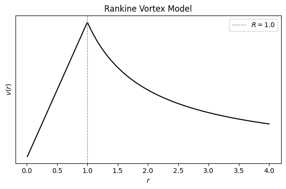
Figure 1: Sketch of the Rankine tangential velocity profile.
2.2 Burgers-Rott model
Later, in 1948, J. M. Burgers showed that there existed a more physically accurate model of vortices [2]. In 1958, N. Rott improved on Burgers’ work and gave us the Burgers-Rott model [7, 3]:
$$ v(r) = \dfrac{\Gamma}{2\pi r}\left(1 - e^{-\alpha\rho r^2/2\mu}\right), \tag{1}\label{burgers} $$where $\rho$ is the density of the fluid, $\mu$ is its viscosity, and $\alpha$ is a constant. Unlike the Rankine model, the Burgers-Rott model also provides radial and vertical velocities ($u = -\alpha r$, $w = 2\alpha z$), making it more physically realistic. Also notice that there is a more realistic transition at the boundary of the vortex (Figure 2). These two improvements to Rankine’s model make the Burgers-Rott model a better candidate for accurately describing tornado vortices. An even better candidate is the Arsen’yev model, which we introduce next.
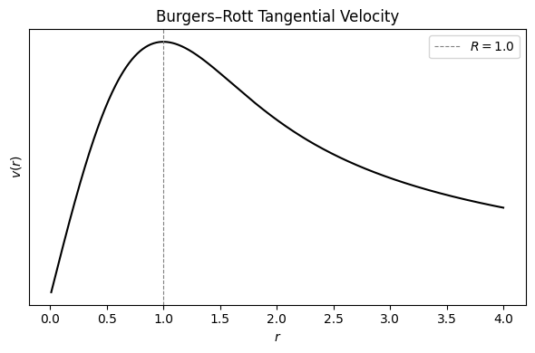
Figure 2: Sketch of the Burgers-Rott tangential velocity profile.
2.3 Arsen’yev model
The Rankine and Burgers-Rott models treat a vortex as an abstract flow; neither one accounts for the specific forces that drive a tornado. Arsen’yev’s approach is different: it starts from the radial acceleration of air and builds in ground friction, turbulent dissipation, and the vertical structure of the storm from the outset [4]. The price of this realism is a longer derivation, but the payoff is a velocity profile that can be compared directly to radar measurements of real tornadoes.
Setting up the equation of motion
The derivation begins by integrating the radial acceleration $\partial u/\partial t$ over the height of the tornado, from the ground up to the top of the storm. This produces a single quantity $S$ that adds up all the inward (or outward) air motion across the full height of the vortex at a given radius. In other words, $S$ tells us how strongly air is being pulled inward at that radius.
Arsen’yev showed that $S$ satisfies the following equation of motion [4]:
$$ \frac{\partial S}{\partial t} = \frac{gh}{c}\frac{\partial S}{\partial r} + \alpha S^2 - f S + A_H \frac{\partial^2 S}{\partial r^2}, \tag{2}\label{dsdt} $$where $c$ is the wave speed and $g$ is the gravitational constant. Each term on the right hand side plays a distinct physical role. The first term, $(gh/c)\,\partial S/\partial r$, describes how the radial flow carries disturbances outward from the vortex core. The $\alpha S^2$ term represents an amplification caused by friction between the tornado and the ground ($\alpha$ is proportional to this friction). On its own, this term would cause the flow to grow without limit, but it is held in check by the damping term $-fS$, where $f$ is related to drag at the top of the tornado. When $S = 1$ these two forces balance; when $S > 1$ the amplification wins. The final term, $A_H\,\partial^2 S/\partial r^2$, represents spreading. The coefficient $A_H$, sometimes called the eddy viscosity, measures how effectively turbulence smooths out differences in the radial flow from one radius to the next [10].
Reducing to an ordinary differential equation
We look for a wave-like solution of the form $S = F(\chi)$ where $\chi \equiv r + ct$. Plugging this into $\eqref{dsdt}$ turns the partial differential equation into an ordinary differential equation (ODE) in $F$. For this to work (for the solution to travel outward as a wave without growing or shrinking), the wave speed must be $c = \sqrt{gh}$. At this particular speed the first term on the right hand side of $\eqref{dsdt}$ cancels exactly, leaving a balance between friction, damping, and spreading [11]. The resulting ODE is
$$ A_H F'' + \alpha F^2 - fF = 0. \tag{3}\label{ode1} $$This equation balances three effects: spreading ($A_H F''$), frictional amplification ($\alpha F^2$), and damping ($fF$). The spreading smooths the profile out, while the push and pull between the other two terms determines how tall the peak is.
Solving the ODE
A useful trick for ODEs like this is to multiply both sides by $F'$. When we do, every term can be written as a derivative of something, which means we can integrate the whole equation in one step. This reduces the problem to a simpler, first-order ODE that we can solve by separating variables.
Defining $\beta \equiv 3f/2\alpha$ (which controls how large the solution can get) and carrying out the integration, we use the identity $\tanh^2(x) = 1 - \operatorname{sech}^2(x)$ to arrive at an explicit formula for $S$:
$$ S = \beta \operatorname{sech}^2\left( \frac{\chi}{\Delta} \right), \tag{4}\label{sech} $$where $\Delta \equiv \sqrt{6A_H/\alpha\beta}$ controls how wide the velocity profile is. The $\operatorname{sech}^2$ function peaks sharply at the centre and drops off to zero on both sides, like a bell curve but with steeper tails. This tells us that the inward-pulling air is concentrated in a narrow band around the vortex core and dies off quickly with distance.
From radial flux to tangential velocity
The quantity $S$ describes the radial momentum, but what we really want is the tangential velocity $v(r)$. To connect the two we need one more physical relationship: inside the tornado, the pressure pushing air inward is balanced by the outward push from the spinning motion. This balance is expressed as
$$ \frac{\partial p}{\partial r} = \rho \frac{v^2}{r}, \tag{5}\label{dpdr} $$where $p$ is the air pressure and $\rho$ is the air density [4]. This says that at every radius, the inward pressure is exactly what is needed to keep the air moving in a circle (this is the same reason why water keeps spinning in a whirlpool).
We also need the relationship between pressure and height: $p = p_0 + \rho g(z - \zeta)$, where $p_0$ is the pressure at ground level. Arsen’yev showed that $\zeta = S/c$, so we can plug in our $\operatorname{sech}^2$ solution for $S$ to get the pressure at the top of the tornado [4]. From there, we take the derivative with respect to $r$, substitute into $\eqref{dpdr}$, and solve for $v$:
$$ \boxed{v(r) = \operatorname{sech}\left( \frac{r + ct}{\Delta} \right) \sqrt{\frac{2g\beta}{c\Delta}\, r \tanh\left( \frac{r + ct}{\Delta} \right)}} $$This gives the tangential velocity at radius $r$ and time $t$. A few things are worth noting about the equation. The $\operatorname{sech}$ factor out front makes the velocity drop off quickly far from the centre, which matches how tornadoes work: the intense winds are concentrated in a small area. The $\sqrt{r\,\tanh}$ factor forces the velocity to zero right at the centre ($r = 0$) and creates a peak at the edge of the vortex, just as we see in real tornadoes. Finally, the parameter $\Delta$ controls how sharp that peak is: a tornado with more internal turbulence (larger $A_H$) has a wider, more gradual velocity peak.
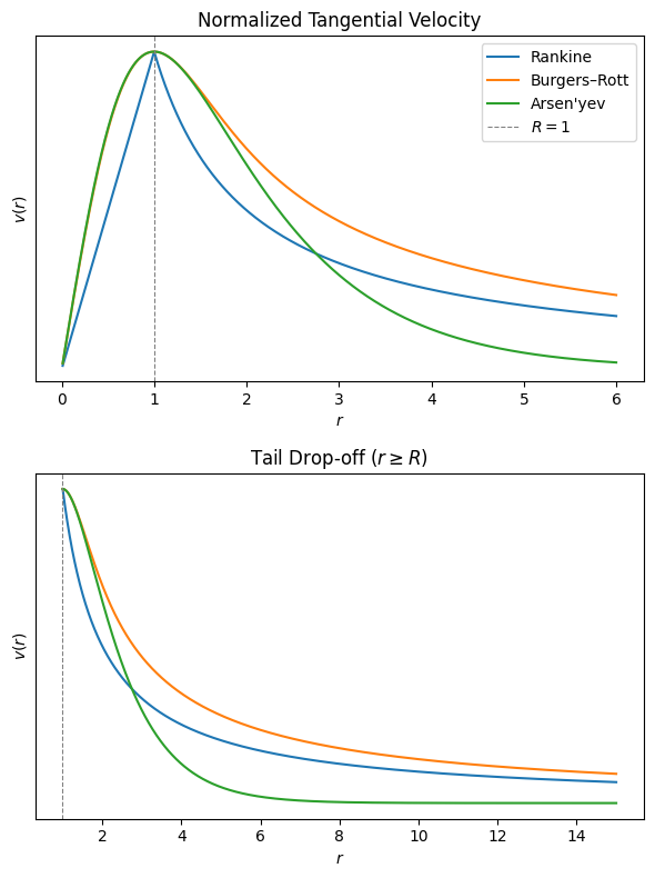
Figure 3: Normalized tangential velocity profiles of all three models (top) and a zoomed view of the tail behaviour for $r \geq R$ (bottom).
The bottom panel of Figure 3 highlights a key difference between the models. Both the Rankine and Burgers-Rott models decay as $1/r$ outside the vortex, which means that wind speeds remain noticeably nonzero even far from the core. The Arsen’yev model, by contrast, inherits an exponential decay from its $\operatorname{sech}$ factor, so the velocity drops to near zero within just a few vortex radii. This faster drop-off is more physical: the force of real tornadoes are tightly concentrated around the vortex and die off rapidly with distance. The leftover velocities predicted by the simpler models are an artifact of their mathematical construction, not something physical.
3. Discussion
The velocity profiles of the Mulhall tornado reveal a clear and consistent structure across altitudes (Figure 4). At every level, the tangential wind rises steeply from near zero at the centre, reaches a sharp peak around $r \approx 0.5$ km, and then decays gradually with increasing radius. The peak velocity varies strongly with height, from roughly 78 m/s near the surface (50 m AGL) down to about 29 m/s at 950 m AGL, showing how vortex winds get stronger close to the ground where surface drag concentrates angular momentum. This alone shows why single-level models are only a first approximation to the full three-dimensional structure of a tornado.
![Figure 4: Mean tangential wind profiles of the Mulhall, Oklahoma tornado at four altitudes (data from Lee and Wurman [5], Figure 5a).](/math/tornadoes/mulhall.png)
Figure 4: Mean tangential wind profiles of the Mulhall, Oklahoma tornado at four altitudes (data from Lee and Wurman [5], Figure 5a).
When the Arsen’yev model is fit to the height-averaged profile, it captures the broad shape of the observed velocity field reasonably well (Figure 5). In particular, the model’s exponential outer decay matches the data closely for $r \gtrsim 1$ km, confirming that the $\operatorname{sech}$ factor is a good description of how tornado winds fall off with distance. However, the model underestimates the peak velocity, reaching approximately 44 m/s compared to the observed average peak of roughly 54 m/s, and places that peak at a larger radius ($r \approx 0.9$ km) than the data ($r \approx 0.5$ km). The inner region, where the wind rises from zero to its maximum, is therefore not well captured. This mismatch is likely because of height averaging: because the peak velocity is much higher near the ground than aloft, the averaged profile has a lower, broader peak that is harder for the model to reproduce with a single parameter set.
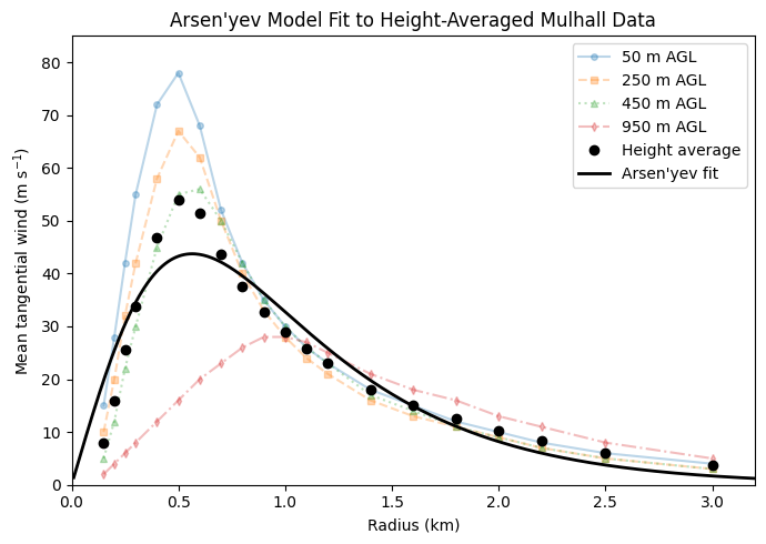
Figure 5: Arsen’yev model fit to the height-averaged tangential wind profile of the Mulhall tornado. The model matches the outer velocity decay well but places the peak at a larger radius than the observations.
These results suggest that the Arsen’yev model is a useful but incomplete description of tornado vortex structure. Its derivation assumes a vertically integrated, axisymmetric flow, which smooths out the strong height dependence observed in the Mulhall data. A better comparison would require fitting the model independently at each altitude, or extending the framework to account for the vertical wind profile. Despite these limitations, the Arsen’yev model is a clear improvement over the Rankine and Burgers-Rott models. It is the only one of the three that correctly predicts a rapid, exponential decay of wind speed outside the core, a feature that is physically real and matters for estimating damage potential and how far dangerous winds extend from a tornado.
References
[1] W. J. Rankine. A Manual of Applied Mathematics. Charles Griffon, London, 1882.
[2] J. M. Burgers. A mathematical model illustrating the theory of turbulence. Advances in Applied Mechanics, 1:171–199, 1948.
[3] N. Rott. On the viscous core of a line vortex. Zeitschrift für angewandte Mathematik und Physik ZAMP, 9(5–6):543–553, 1958.
[4] S. A. Arsen’yev. Mathematical modeling of tornadoes and squall storms. Geoscience Frontiers, 2(2):215–221, 2011.
[5] W.-C. Lee and J. Wurman. Diagnosed three-dimensional axisymmetric structure of the Mulhall tornado on 3 May 1999. Journal of the Atmospheric Sciences, 62(7):2373–2393, 2005.
[6] R. Rotunno. The fluid dynamics of tornadoes. Annual Review of Fluid Mechanics, 45:59–84, 2013.
[7] K. Kilty. Steady-state tornado vortex models. Kilty’s Office, pp. 1–14, 2005.
[8] B. Khouider. Class Notes: Waves in the Atmosphere and the Ocean, pp. 32–34. University of Victoria, 2018.
[9] G. J. Holland. An analytic model of the wind and pressure profiles in hurricanes. Monthly Weather Review, 108(8):1212–1218, 1980.
[10] B. Khouider. Personal interview. December 13, 2018.
[11] B. Khouider. Email conversation. December 16, 2018.