Modelling influenza spread on contact networks using a SIRS-Miller framework
Brody Reid —
Updated on
Originally written April 2019. This version has been revised to use a SIRS framework, a negative binomial degree distribution, and a Python implementation. The original analysis and its limitations are discussed in Section 6.
Abstract: The Miller model draws on contact networks, probability theory, and infectious-disease dynamics to describe how a disease spreads through a population. We model the population as a network where each person is a node and each social connection is an edge. We work within the susceptible-infected-recovered-susceptible (SIRS) framework, which accounts for the fact that immunity to influenza is temporary, and assume a negative binomial degree distribution for the network (a choice supported by empirical contact survey data [5]). We fit the model to the CDC’s weighted percentage of influenza-like illness (ILI) visits from the 2017–2018 season using an observation model with a scaling parameter and a baseline ILI rate. The fitted model captures the overall shape of the epidemic curve well, with a transmission rate $\beta \approx 0.47$ per day, an implied mean degree of $\langle k \rangle \approx 1.49$, and a background ILI baseline of approximately 1%. We discuss the model’s performance and remaining limitations.
AI Disclosure
This paper was revised with writing assistance from Claude (Anthropic), accessed via Claude Code. The AI was used to help rewrite and improve the clarity of the text. All mathematical content, analysis, and conclusions are the author’s own. The final version was reviewed and edited by Brody Reid.
1. Introduction
Classical epidemic models assume a well-mixed population, where every individual is equally likely to encounter every other. In reality, disease spreads along specific social connections, and the structure of those connections shapes how quickly and widely an outbreak can travel. In 2011, Joel C. Miller formalized this idea in a framework that builds SIR-type dynamics directly on top of a contact network [1], allowing the heterogeneity in people’s social connections to influence transmission.
Here, we test an extended version of Miller’s model against data from the Centers for Disease Control and Prevention [2]: the weighted percentage of outpatient visits for influenza-like illness (ILI) reported through the ILINet surveillance system over the 2017–2018 season. Two key choices distinguish this analysis from a basic SIR-Miller model. First, we use a SIRS framework: for influenza, immunity is strain-specific, and a person who recovers from one circulating strain can still be infected by another, so treating recovery as permanent is unrealistic. Second, we model the distribution of contacts using a negative binomial distribution rather than a Poisson, which better reflects the heterogeneity actually observed in social networks [5].
2. Contact Networks
A contact network represents a population as a graph. Each person is a node, and each social connection through which infection could spread is an edge. The number of edges connected to a given node is called its degree, denoted $k$. People with many contacts have high degree; people with few have low degree.
The distribution of degrees across the population is described by $P(k)$, the probability that a randomly chosen person has exactly $k$ contacts. The average number of contacts per person is:
$$\langle k \rangle = \sum_{k=1}^\infty k\, P(k). \tag{2.1}$$A useful mathematical object for working with degree distributions is the probability generating function:
$$\psi(x) = \sum_{k=0}^\infty P(k)\, x^k. \tag{2.2}$$This encodes the entire degree distribution in a single function and makes later calculations more compact. One handy property: the average degree is simply the derivative of $\psi$ evaluated at $x = 1$, i.e., $\langle k \rangle = \psi'(1)$.
To make this concrete, imagine a workplace where most employees interact with a small team daily, a few managers coordinate across several teams, and one or two highly connected individuals seem to know everyone. Suppose 60% of people have 3 regular contacts, 30% have 8, and 10% have 20. The average degree is $\langle k \rangle = 0.6(3) + 0.3(8) + 0.1(20) = 6.2$, but this average masks a wide spread; the small group of highly connected individuals contributes disproportionately to how quickly an infection can move through the network.
3. The SIRS Model
The SIRS model extends the classic SIR model by adding a pathway from recovered back to susceptible. The population is divided into three groups:
- Susceptible $S(t)$: people who could catch the disease.
- Infected $I(t)$: people who currently have it and can spread it.
- Recovered $R(t)$: people who have recovered and are temporarily immune.
Susceptibles become infected at rate $\beta$ through contact with infected individuals. Infected individuals recover at rate $\gamma$. Recovered individuals lose their immunity and return to the susceptible pool at rate $\delta$. In a population of $N$ people, the dynamics are [3]:
$$\dot{S} = -\beta SI + \delta R, \tag{3.1}$$$$\dot{I} = \beta SI - \gamma I,$$$$\dot{R} = \gamma I - \delta R.$$The $\delta R$ term is the key addition: rather than leaving the recovered pool permanently, individuals cycle back into the susceptible pool as immunity wanes. For influenza, $\beta \approx 0.06$ per day and $\gamma \approx 0.2$ per day [4]. For the waning immunity rate we use $\delta = 1/365$ per day, reflecting roughly one year of strain-specific immunity.
4. The Miller Model
Miller’s model builds the SIR framework on top of a contact network, so that the structure of social connections shapes how the disease spreads [1]. Here we extend it to accommodate SIRS dynamics and a negative binomial degree distribution.
4.1 Core Network Variables
The model tracks two network-level probabilities:
- $\theta(t)$: the probability that a randomly chosen edge has not yet transmitted the infection by time $t$.
- $\varphi(t)$: the probability that the person at one end of a randomly chosen edge is currently infected, but has not yet passed the infection along that edge.
Think of $\theta$ as measuring how much of the network is still “unexposed,” and $\varphi$ as capturing the active transmission pressure on any given connection. As time passes, $\theta$ falls as transmission occurs and $\varphi$ evolves according to how quickly infected nodes recover versus how quickly they infect their neighbours.
4.2 Negative Binomial Degree Distribution
Empirical contact surveys consistently show that the number of social contacts per person is overdispersed: the variance is much larger than the mean, with a long tail of highly connected individuals [5]. A Poisson distribution cannot capture this, since for Poisson the variance equals the mean. The negative binomial distribution adds a second parameter that controls how spread out the distribution is, making it a much better match to observed contact patterns.
The negative binomial has parameters $n > 0$ (a shape parameter controlling overdispersion) and $0 < p < 1$ (related to the mean number of contacts). The probability of having exactly $k$ contacts is:
$$P(k) = \binom{k+n-1}{k} (1-p)^n p^k, \tag{4.1}$$with mean $\langle k \rangle = np/(1-p)$ and variance $np/(1-p)^2$. When $n$ is large the distribution approaches Poisson; when $n$ is small the tail is heavy and a few highly connected individuals dominate.
The probability generating function is [6]:
$$\psi(x) = \left(\frac{1-p}{1-px}\right)^n. \tag{4.2}$$Its first and second derivatives, which appear in the Miller equations, are:
$$\psi'(x) = \frac{np(1-p)^n}{(1-px)^{n+1}},$$$$\psi''(x) = \frac{n(n+1)p^2(1-p)^n}{(1-px)^{n+2}}.$$Evaluating at $x = 1$ gives the mean: $\psi'(1) = np/(1-p)$.
4.3 The Full SIRS-Miller System
Extending the Miller model to SIRS requires an additional variable, $\varphi_R(t)$: the probability that the base node of a random edge is currently recovered and the edge has not transmitted. Under the approximation that re-susceptible individuals re-enter the network fresh (i.e., their edges are again available for transmission), the system is:
$$\dot{\theta} = -\beta\varphi, \tag{4.3}$$$$\dot{\varphi} = -(\beta + \gamma)\varphi + \beta\varphi\cdot\frac{\psi''(\theta)}{\psi'(1)}, \tag{4.4}$$$$\dot{\varphi}_R = \gamma\varphi - \delta\varphi_R, \tag{4.5}$$$$\dot{I} = N\beta\varphi\,\psi'(\theta) - \gamma I, \tag{4.6}$$$$\dot{R} = \gamma I - \delta R. \tag{4.7}$$Substituting the negative binomial expressions for $\psi'(\theta)$ and $\psi''(\theta)/\psi'(1)$:
$$\psi'(\theta) = \frac{np(1-p)^n}{(1-p\theta)^{n+1}},$$$$\frac{\psi''(\theta)}{\psi'(1)} = \frac{(n+1)p(1-p)^{n+1}}{(1-p\theta)^{n+2}}.$$The initial conditions are $\theta(0) = 1$, $\varphi(0) = I_0/N$, $\varphi_R(0) = 0$, $I(0) = I_0$, $R(0) = 0$.
4.4 Observation Model
The SIRS-Miller system produces absolute incidence, $N\beta\varphi\,\psi'(\theta)$ new infections per day, but the CDC ILINet data reports the weighted percentage of outpatient visits attributable to influenza-like illness (% Weighted ILI). These are fundamentally different quantities: the model output scales with the total population $N$, while the surveillance data is a proportion of clinic visits.
To bridge this gap, we express the model’s incidence as a fraction of the population,
$$f(t) = \beta\varphi\,\psi'(\theta) = \frac{\beta\varphi\, n p(1-p)^n}{(1-p\theta)^{n+1}}, \tag{4.8}$$and introduce two additional parameters. The first is a scaling parameter $\rho$, which absorbs the proportionality between the true per-capita infection rate and the fraction of outpatient visits coded as ILI. The second is a baseline $b$, representing the background rate of ILI visits from non-influenza respiratory pathogens (rhinovirus, RSV, etc.) that persists year-round. The observation model is then:
$$\text{\% Weighted ILI}(t) \approx \rho\, f(t) + b. \tag{4.9}$$This formulation avoids the need to estimate the absolute number of infections. The five fitted parameters are $\beta$, $n$, $p$, $\rho$, and $b$; the remaining parameters $\gamma$, $\delta$, and $I_0$ are fixed from the literature.
5. Analysis
We fit the observation model (4.9) to CDC ILINet data for the 2017–2018 influenza season [2], which consists of 52 weekly observations of % Weighted ILI. The season runs from MMWR week 40 of 2017 through week 39 of 2018. We set $\gamma = 0.2$ per day (5-day average infectious period) and $\delta = 1/365$ per day (one year of strain-specific immunity) based on the literature [4]. The initial infected count is $I_0 = 12{,}839$, taken from the first week’s reported ILI total, and $N = 327{,}200{,}000$.
The system of ODEs (4.3)–(4.7) is integrated numerically using a fourth-order Runge–Kutta method (RK45) with relative tolerance $10^{-6}$ and absolute tolerance $10^{-8}$. The observation model $\rho\,f(t) + b$ is then fit to the data by nonlinear least squares (trust-region reflective algorithm), minimizing the sum of squared residuals between the predicted and observed % Weighted ILI at each week.
The fitted parameters and their standard errors are:
| Parameter | Estimate | Interpretation |
|---|---|---|
| $\beta$ | 0.47 | Transmission rate per edge per day |
| $n$ | 50.0 | Negative binomial shape (overdispersion) |
| $p$ | 0.029 | Negative binomial success probability |
| $\rho$ | 41.7 | Scaling from infection rate to ILI% |
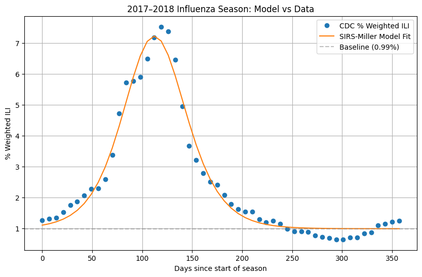
| $b$ | 0.0099 | Baseline ILI rate (0.99%) |
The implied mean degree is $\langle k \rangle = np/(1-p) \approx 1.49$, and the large fitted value of $n$ means the degree distribution is only weakly overdispersed, close to Poisson. The baseline of approximately 1% is consistent with the off-season ILI activity typically reported by ILINet.
The model captures the overall shape of the 2017–2018 epidemic curve well: the gradual rise from October through December, the sharp peak in late January / early February, and the return to baseline by late spring. The fitted curve slightly underestimates the peak (the model reaches about 7.1% versus the observed peak of 7.5%), and the observed data shows a secondary shoulder around days 140–170 that the single-strain model cannot reproduce. This likely reflects the sequential circulation of influenza A (H3N2) followed by influenza B during that season.
6. Discussion
The model fits the 2017–2018 ILINet data well, capturing the rise from October, the sharp peak in late January / early February, and the return to baseline by late spring. The fitted transmission rate of $\beta \approx 0.47$ per day is higher than the literature estimate of $\approx 0.06$ for a well-mixed population [4], which is expected: in the network model, transmission occurs along edges rather than uniformly, and the relatively low implied mean degree ($\langle k \rangle \approx 1.49$) means a higher per-edge rate is needed to produce the same population-level dynamics. The baseline of $b \approx 1\%$ agrees with the off-season ILI rate typically reported by ILINet, lending confidence that the observation model (4.9) is correctly partitioning influenza-driven and background ILI activity.
The two main modelling choices — switching to SIRS and adopting a negative binomial degree distribution — address what were identified as the most significant shortcomings of a basic SIR-Miller approach.
The negative binomial is a well-motivated choice. Mossong et al. [5], in a large contact survey spanning eight European countries, found that the distribution of daily contact counts is substantially overdispersed, with a long right tail driven by a small number of highly social individuals. A Poisson distribution, where variance equals the mean, cannot represent this; the negative binomial can. In practice, however, the fitted value of $n \approx 50$ suggests the data does not strongly constrain overdispersion for this particular season: with $n$ this large the negative binomial is nearly Poisson.
The SIRS extension is similarly well-motivated for influenza. Because multiple strains co-circulate and the dominant strain shifts each season, strain-specific immunity wanes on a timescale of roughly a year. The $\delta$ parameter captures this, and its inclusion means the model can in principle be fit to multi-season data rather than a single outbreak curve.
Fitting to the weighted ILI percentage rather than raw case counts avoids the need to estimate the absolute number of infections, which is unobservable. The observation model (4.9) introduces just two extra parameters ($\rho$ and $b$), both of which are well-constrained: the baseline $b \approx 1\%$ agrees with the off-season ILI rate typically reported by ILINet, and $\rho$ absorbs the unknown proportionality between the true infection rate and the fraction of outpatient visits coded as ILI.
One limitation that remains is the approximation in Section 4.3: re-susceptible individuals are treated as re-entering the network fresh. In reality, whether a previously-used edge can transmit again depends on the specific immunological history of both nodes. A more rigorous treatment would track edge states explicitly, but this becomes computationally expensive for large networks. For a first-order correction the approximation is reasonable, but it is worth bearing in mind when interpreting fitted parameter values.
The standard errors on $n$ and $p$ individually are large, reflecting a strong correlation between them: many combinations of $n$ and $p$ yield similar mean degrees $\langle k \rangle = np/(1-p)$. Profile likelihood or Bayesian methods would better characterize this joint uncertainty.
A further improvement would be to fit to averaged multi-year incidence data rather than a single season, which would reduce year-to-year noise and give a more stable signal to fit against. A multi-strain extension that tracks influenza A and B separately could also capture the secondary shoulder visible in the 2017–2018 data.
References
[1] Miller, J. C. (2011). A note on a paper by Erik Volz: SIR dynamics in random networks. Journal of Mathematical Biology, 62(3), 349–358, arxiv.org.
[2] Centers for Disease Control and Prevention. Weekly U.S. Influenza Surveillance Report. cdc.gov. Accessed 2026-03-12, season selection: 2017–2018.
[3] Weisstein, E. W. Kermack-McKendrick Model. From MathWorld – A Wolfram Web Resource. mathworld.wolfram.com.
[4] Ma, J., van den Driessche, P., & Willeboordse, F. H. (2013). The importance of contact network topology for the success of vaccination strategies. Journal of Theoretical Biology, 325, 12–21.
[5] Mossong, J., Hens, N., Jit, M., Beutels, P., Auranen, K., Mikolajczyk, R., et al. (2008). Social contacts and mixing patterns relevant to the spread of infectious diseases. PLOS Medicine, 5(3), e74.
[6] Proof Wiki. Probability Generating Function of Negative Binomial Distribution. proofwiki.org. May 2013.
[7] Edwards, R. (2019, April 5). Personal conversation.
[8] Ma, J. (2019, April 1). Personal conversation.